Technical Writing and Publishing Data-Rich Articles with Quarto

Key points

• Highly-technical paper in science and engineering relies on extensive data analysis–this can affect reproducibility.
• Python-based notebooks have long provided the capability of merging the paper narrative, the computational code powering the analysis, and the summary plots into a reproducible report.
• Quarto is a recent addition to the python ecosystem, and provides a streamlined publication procedure. It lowers the adoption barrier of the “docs as code” paradigm.
• With a single command, the notebook text sources (narrative and code) are transformed into a polished publication-ready article in a variety of formats (PDF or dynamic HTML page enabling the reader to interact with the data tables and plots.

Figure 1: Technical writing workflow, starting from plain text (narrative, code and data) all under version control for reproducibility.

Introduction

Technical writing is critical for engineers and scientists to communicate their idea, design, analysis and conclusions. The analysis is typically data and computational intensive. For transparency and reproducibility, the computer code generating the summary tables and plots should be shared along with the narrative. Python-based Jupyter notebooks have long provided the capability of merging the narrative, the code, and the summary plots into an executable report. Another step is needed to format the report for formal publication. In addition, for scholarly articles (“papers”), additional elements are needed such as numbered figures, cross-references, citations, formatted bibliography. These are not available as part of the standard notebooks.

Quarto is a recent addition to the python ecosystem which streamlines the complete publication process. It was launched in July 2022 (see announcement) for Python, but has long been developed for publishing R notebooks. It was specifically designed to generate scholarly articles with all formal elements included. It is based on the Swiss knife of document conversion: pandoc. Hence, it supports multiple outputs formats–see the quarto gallery for multiple examples. In addition to the classical PDF scholarly article, it can also generate modern and dynamic HTML pages, which enable the reader to engage with the data tables and plots to develop his/her own insight.

Quarto handles not just the final formatting but also the execution of the analysis code, generating the tables and plots on the fly. This is done with just one command quarto render. Consequently, the complete article can be re-executed in a matter of seconds during the authoring. This is also helpful for the independent verification by peers. The article and the analysis therein can also be “forked” to start a new branch of analysis by changing the assumptions or data. Hence, Quarto favors reproducibility, transparency, and collaboration.

Related tools

Executable notebooks exist in other languages (matlab, R, Julia, …), but Python is the most popular as per the TIOBE index. Crucially, Python provides an excellent fit for a broad set of activities in microsystems and hardware development, as this blog will demonstrate time and time again. See [1] for a relevant example of system modeling and analysis in Python.

Even within the Python ecosystem, there are similar tools to Quarto. As usual with Python there are multiple ways to realize a task. For notebook publication, nbconvert and jupyterbook are established alternatives, and generate also publication-quality outputs.

Why Quarto ?

Quarto stands out, aesthetically, with its is beautiful modern templates (for books, articles, course notes, blogs, …) out of the box. But they key differentiator is the built-in features for scholarly writing. In that specific niche, it is game changer.

Quarto generates publication-quality articles in various scientific journal templates. See this link for the growing list of supported journal. Again, a single command is needed quarto use template <journal-name>. Blogs are also supported—this blog is built with Quarto. Even complete interactive website and course notes can be generated. See the course Practical Deep Learning for an extensive example, which was used as a pilot for porting Quarto into the Python ecosystem. This short video shows how a minimalistic operational website can be build from plain text and publish online for free in under 60 sec. In summary, Quarto is a battery-included publishing tool chain, with easy configuration and excelling at producing formal articles. See this curated list for additional Quarto resources.

Preview of this article

This article is a walk-through of the capabilities of Quarto. A fictitious data analysis, with data-rich tables and plots, is used to included to demonstrate the features. The sources and resulting PDF and interactive HTML are made available at Github for easy reproduction.

We introduce our Quarto workflow in Section 2. As usual with Python, there could be multiple other options. Section 3 quickly explains how to get started for scholarly writing. Section 4 is a basic data analysis to illustrate how Quarto executes the analysis code on the fly to produce the summary tables and plots. We also highlight the key advantages of publishing to an interactive HTML page, as opposed to a static PDF, enabling the reader to explore on its own the tables and plots. Finally, Section 5 compares side-by-side the PDF and the HTML and discuss the merits of each.

Quarto workflow

Jupyter notebooks can be represented in a variety of related plain text formats (see Jupytext for the full list). These file format defines the syntax for the narrative text (based the most popular plain text format: Markdown), and the Python code. Quarto uses its own Markdown flavor (*.qmd) which provides extensions for scholarly writing.

The workhorse is then the text editor. Given the universality of the plain text format, any editor can be used—you can keep using your favorite ones. This link provides tips for configuring any editor with Quarto and enjoying automatic live rendering in a side window.

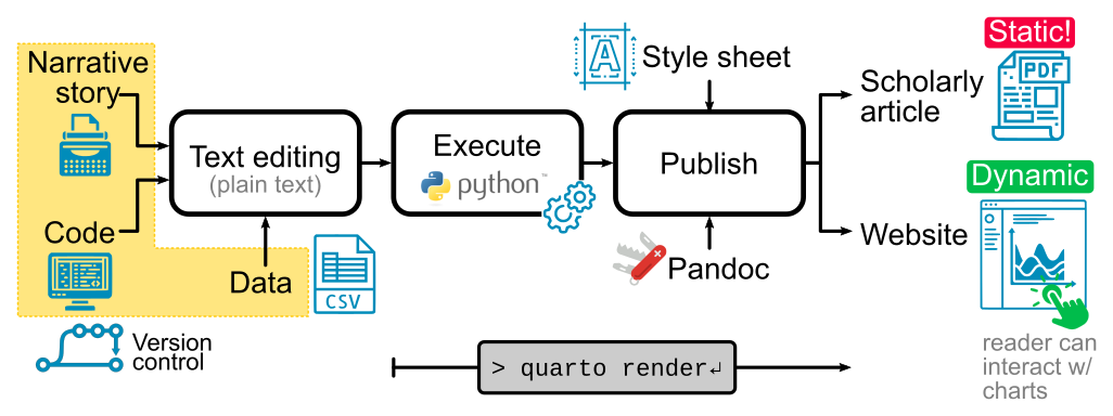
Figure 1 illustrates the workflow. The narrative part is text-edited in markdown, with the python code mixed inside python code cells, delimited by ```{python} markers. The support data would often be in the form of a text file (CSV). All source elements are then editable from the text editor. The polished article (or book or website) is rendered automatically on the side when the source changes.

Important

All elements of the document (narrative, equations, tables, bibliography) apart from the support diagrams are entered in plain text, and they are treated like code. This paradigm is referred as “docs as code”, and is increasingly popular beyond its home ground in software engineering.

The critical advantages are:

• All assets are stored in the universal computer format: plain text files. They can be edited by any text editor, and readily shared and reused. This is unlike contents that is trapped in proprietary formats, which invariably needs to be copy and pasted then reformatted.

• The text files are effectively managed by a version control system, next to the code and other files. This ensures consistency between the pure code and document elements, through the multiple revisions and multiple contributors. Changes from multiple contributors can be merged, in a controlled fashion, inherited from rigorous software practices.

When the sources file are shared with the readers, the resulting article paper is then “executable”. A formal definition of an executable article is given in [2].

executable article/paper [definition]

scientific paper enabling the reader to reproduce each and every step in to arrive at paper conclusions, from the raw data to the polished plots.

Note that the emphasis is on the final polished tables and plots, not just the interim visuals found in the supplementary materials. These are separated from the final tables and plots, and don’t show the exact steps to reproduce the final plots and tables supporting the conclusions.

Walk-through

To get started, install Quarto as per the instructions and check the tutorial. Start drafting your article in a file article.qmd.

Quarto, like many other Markdown-based tools, handles naturally the usual technical writing elements. Figures, tables, in-line equation, block equations, and code listings are all supported. These are the core building blocks of technical writing. These elements are part of basic Markdown, and not specific to Quarto. On the other end, captions and cross-references are not part of basic Markdown. Quarto supports them out of the box, along with other features for scholarly writing, such as title block, appendices, and other metadata to make the article citeable. The metadata is added in the article front-matter as YAML key-value pair. From the default configuration, one adds the title, author, date, abstract, bibliography, license and some HTML and PDF formatting options, then one starts writing the text and coding the code cell. Here is a bare-bones article.qmd to get started.

Technical writing elements

Quarto, like many other Markdown-based tools, handles naturally the usual technical writing elements. Figures, tables (see Table 1), in-line equation (e.g. \(r=\sqrt{x^2+y^2}\)), block equations, and code listings are all supported. These are the core building blocks of technical writing.

Table 1: Table of sensor parameters

Parameter	Symbol	Min	Typ	Max	Unit
Supply current	\(i_\text{off}\)	-	-	10	mA
Hall sensitivity	\(S_\text{H}\)	0.2	-	-	V/T
Effective number of bits	\(\text{ENOB}\)	12	-	-	-

Block of Latex-formatted equations are also supported.

\[ \begin{aligned}\nabla \times \vec{\mathbf{B}} -\, \frac1c\, \frac{\partial\vec{\mathbf{E}}}{\partial t} & = \frac{4\pi}{c}\vec{\mathbf{j}} \\ \nabla \cdot \vec{\mathbf{E}} & = 4 \pi \rho \\\nabla \times \vec{\mathbf{E}}\, +\, \frac1c\, \frac{\partial\vec{\mathbf{B}}}{\partial t} & = \vec{\mathbf{0}} \\\nabla \cdot \vec{\mathbf{B}} & = 0 \end{aligned} \tag{1}\]

These elements are part of basic Markdown, and not specific to Quarto. On the other end, captions and cross-references (such as Table 1, Equation 1) are not part of basic Markdown. Quarto supports them out of the box, along with other features for scholarly writing, such as title block, appendices, and metadata to make the article citeable.

Executable code

The real power of Quarto (and the underlying Jupyter notebooks) is the ability to combine narrative text, explaining the story, with executable code to recompute on the fly and display tables and plots. As an example, we use a classical dataset from 1993 compiling physical and performance characteristics of hundreds of cars (weight, cylinders, power, mileage, acceleration). It is available there. The table below displays the first 5 rows of the dataset.

Note that this code invokes some boilerplate initialization code. The Python dependencies are listed in requirements.txt.

Code

from bokeh.sampledata.autompg import autompg_clean as df
interesting_cols = ['name', 'origin', 'hp', 'mpg', 'weight']
from tabulate import tabulate

Code

Markdown(tabulate(df.head(5)[interesting_cols], headers='keys', showindex=False))

Table 2: Dataset preview

name	origin	hp	mpg	weight
chevrolet chevelle malibu	North America	130	18	3504
buick skylark 320	North America	165	15	3693
plymouth satellite	North America	150	18	3436
amc rebel sst	North America	150	16	3433
ford torino	North America	140	17	3449

Such raw table just shows the dataset structure, but does not inform much the reader—it does not depict an underlying trend (and it lacks units). We will improve these weaknesses later by manipulating the raw table in Python using the outstanding pandas library (see also the open-access book Python for Data Analysis for using this library in a practical data analysis). Incidentally, the web-version of the book was also created with Quarto.

Let’s say, for the sake exercising the Quarto workflow in a dummy analysis, we are interested in shortlisting cars with high mileage and high power, and we speculate that these two are in conflicts. To visualize the trade-off, we plot both these characteristics in a scatter plot. We color the point with the continent of origin.

Code

ax=sns.scatterplot(data=df.dropna(), x='mpg', y='hp', hue='origin')
ax.set(xlabel='Mileage [mpg]', ylabel='Power [hp]'); #explicit semicolomn to hide output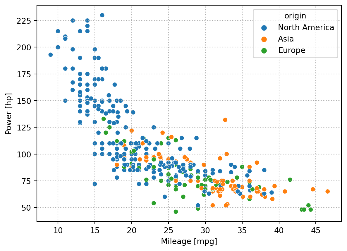

Trade-off curve showing the conflict between high mileage and high power.

Two trends are visible:

1. There is a trade-off between power and mileage (a classic trade-off in engineering between performance and resources needed).
2. European and Asian cars tend to offer higher mileage.

The second trend can be also summarized in a pivot table. The pivot table operator in pandas provides a concise yet readable syntax, making the intent clear in the code. Here we summarize the dataset by taking the average mileage and power per continent of origin.

Code

df2=pd.pivot_table(
  data=df,
  values=['mpg', 'weight'],index=['origin'],aggfunc='mean')

Markdown(tabulate(df2, headers='keys'))

origin	mpg	weight
Asia	30.4506	2221.23
Europe	27.6029	2433.47
North America	20.0335	3372.49

Finally, let’s say that we now focus on just 10 cars with the highest mileage. It is then practical to list them all. In addition to manipulating the numbers, pandas can also manipulate the style of the table. The styling is applied when rendering to a HTML page. To obtain the same rendering in the PDF, we treat the rendered table as a figure by exporting the rendered table to an image using the dataframe-image library. Here we sort the table by mileage (by descending order), highlight the extremes in weight in red and green, and add an inline bar chart for power.

Code

import dataframe_image as dfi

# Add unit
df2=df[['name', 'origin', 'hp', 'weight', 'mpg']].sort_values(by='mpg', ascending=False).head(10).set_index(['name', 'origin'])
df2.rename(columns={
  'hp':     'power [hp]',
  'weight': 'weight [lbs]',
  'mpg':    'mileage [mile/gallon]'
  }, inplace=True
)
df2.columns = pd.MultiIndex.from_tuples(df2.columns.str.extract('(.*) \[(.*)\]').to_records(index=False).tolist())


# Export styled table
try:
  dfi.export(
  df2.style.bar(subset=["power"], color='#0095B6').\
        format(precision=0, thousands=" ").\
            highlight_max(subset='weight', color='orangered').\
              highlight_min(subset='weight', color='green').\
                set_table_attributes(my_table_class),
    "_outputs/shortlist.png")
except:
  pass

Code

Image('_outputs/shortlist.png', width=500)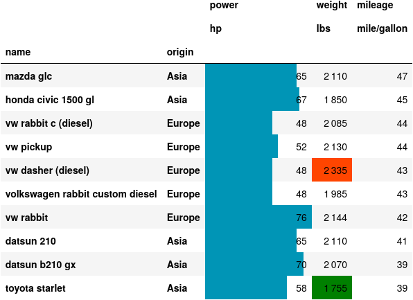

Figure 2: Short list of cars

Based on our criteria, we select, among the 10 cars the highest mileage, the car providing the highest power: the VW rabbit. Note that we can also embed calculated expression in text. As an example, we summarize below the characteristics of the VW rabbit, programmatically converted by the Pint library into standard units.

Code

# Define new unit: liter per 100 km
ureg.define('liter_per_100km = liter/( 100 * km) = l/100km')
ureg.default_format = '~.1f'

# Conversion
df2=df2.pint.quantify()
df2['consumption']=1/df2.mileage
df2.consumption=df2.consumption.pint.to('liter_per_100km')
df2.power=df2.power.pint.to('kW')
df2.weight=df2.weight.pint.to('kg')
vw_rabbit=df2.loc["vw rabbit",:].iloc[0]

Markdown(f"The VW rabbit delivers {vw_rabbit.power:~.1f}, \
  consumes {vw_rabbit.consumption:~.1f} and \
  weights {vw_rabbit.weight:~.1f}.")

The VW rabbit delivers 56.7 kW, consumes 5.7 l/100km and weights 972.5 kg.

HTML only

In HTML webpage, as opposed to static PDF, the document can be interactive. Instead of the static plots and table as above, we can share with the reader interactive versions. The panel library supports interactive plots, tables via the tabulator widget, and the composition of dashboard.

The interactive features of plots include tooltips, filtering, zooming, … The tables can also be made lively with filtering, sorting … Large data table with hundreds of records can also be displayed thanks to the table scrolling feature. These interactive features favor self-exploration by the readers, developing new insight into the audience. An interactive dashboard is shown below, by combining the key trade-off curve and the table.

Code

hv.extension('bokeh')
import panel as pn
pn.extension('tabulator', css_files=[pn.io.resources.CSS_URLS['font-awesome']])


p=df.hvplot.scatter(x='mpg', y='hp', groupby='origin',
  hover_cols=['name'],
  width=600)

# Alternative
# t=hv.Table(df[interesting_cols]).opts(width=600)
filters = {
    'name':   {'type': 'input', 'func': 'like'},
    'origin': {'type': 'input', 'func': 'like'},
    # Filter based on min threshold
    #'hp': {'type': 'number', 'func': '>=', 'placeholder': 'min'}
}

t=pn.widgets.Tabulator(
     df[interesting_cols],   
     sizing_mode="stretch_width",
     show_index=False,
     header_filters=filters, #header_filters=True, 
     page_size=10,
     height=600)

pn.extension('tabulator', css_files=[pn.io.resources.CSS_URLS['font-awesome']])
pane=pn.Column(p,t)
pane.embed()

The interactivity in HTML also allow advanced layout such as tabs and lightbox to show galleries of images.

Conclusion

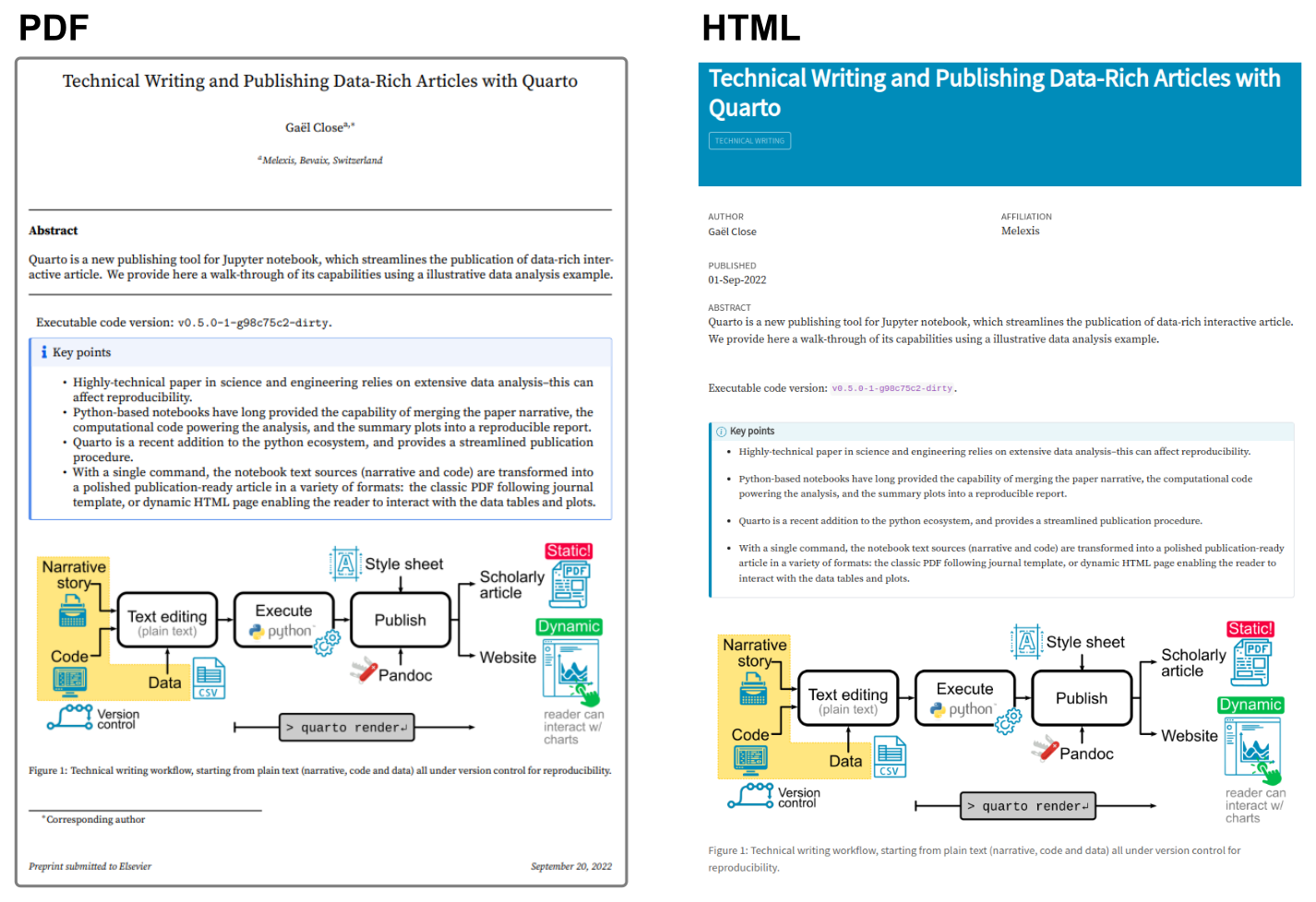
With a single command quarto render <file>, Quarto produces publication-ready PDF and interactive HTML from the same source. Either of the outputs can be readily shared and published. The HTML can be hosted on a public or internal server, as a standalone article or as part of complete website. Thanks to the interactivity, this is the preferred format. The HTML is published on the author’s blog. The static PDF, could be uploaded to a pre-print server such as TechRxiv or arxiv, thereby obtaining an official DOI, and preserving the PDF for decades to come. In this case the PDF is published on author’s Research Gate profile, and is citeable.

• G. Close, “Technical Writing and Publishing Data-Rich Articles with Quarto,” Research Gate, 20-Sep-2022. Available: http://dx.doi.org/10.13140/RG.2.2.14862.43846/1

The first page of each output is shown in Figure 3 illustrating the consistency. Again such results are also possible with nbconvert and jupyter-book. Quarto shines with the relative ease of configuration, which lowers the barrier to adoption for the “docs as code” paradigm.

Figure 3: Generated PDF and HTML side-by-side.

Overall, Quarto is a battery-included publications tool chain, generating high-quality modern scholarly articles with just one command and minimal configuration. It is a solid alternative to nbconvert and jupyter-book, worth considering for technical writers contemplating a move to the “docs as code” paradigm. This paradigm is not for everyone (see this article for the challenges), as this is still code heavy. But Quarto makes it more accessible.

Appendix

VSCode extensions

Any text editor can be used to edit the plain text files. That being said, VSCode provides an ideal environment for technical writing with Quarto. VSCode is natively well suited to develop Python code (executing code on the side, navigating the code base …). This article provides tips to get started with technical writing in VSCode (installing basic spell check, git integration, …). Then the Quarto VScode extension can trigger the Quarto rendering/previewing directly from the editor. Two extra extensions vscode-data-preview and gc-excelviewer allow the take a sneak preview at the data files (CSV or Excel files) directly from the editor. Thanks to above extensions, the technical writing productivity is supercharged into a different league with respect to traditional writing in Microsoft Word or Google Doc.

Exploratory data analysis library

In the above analysis, we quickly jumped into a dedicated analysis. In practice and for new dataset, it might be wiser to explore the dataset more thoroughly to get familiar with the data structure and correlation. The pandas-profiling library is ideal for first exploration. With a few lines of code, it generates an extensive report containing the histograms of values for each column, and the correlations between any pair of columns. The following code generates such a report.

```{python}
from pandas_profiling import ProfileReport
profile = ProfileReport(df, title="Pandas Profiling Report")
profile.to_file("../../resources/profile-report.html")
```

Watermark

Code

%load_ext watermark
%watermark -n -u -v -g -iv

The watermark extension is already loaded. To reload it, use:
  %reload_ext watermark
Last updated: Mon May 01 2023

Python implementation: CPython
Python version       : 3.9.12
IPython version      : 8.4.0

Git hash: 2cf6d41e5b1430ef5752aeec2fe91e39d3a895bf

pint_pandas    : 0.2
dataframe_image: 0.1.2
matplotlib     : 3.5.3
forallpeople   : 2.6.3
pandas         : 1.4.4
sys            : 3.9.12 (main, Apr  5 2022, 06:56:58) 
[GCC 7.5.0]
seaborn        : 0.11.2
holoviews      : 1.15.0
pyprojroot     : 0.2.0
hvplot         : 0.8.1
panel          : 0.13.1
logging        : 0.5.1.2
numpy          : 1.23.5

References

[1]

G. Close, “Signal chain analysis in python: A case study for hardware engineers.” Feb. 2021 [Online]. Available: https://towardsdatascience.com/signal-chain-analysis-in-python-84513fcf7db2

[2]

J. Lasser, “Creating an executable paper is a journey through open science,” Communications Physics, vol. 3, no. 1, pp. 1–5, Aug. 2020 [Online]. Available: https://www.nature.com/articles/s42005-020-00403-4

Reuse

Citation

BibTeX citation:

@online{close2022,
  author = {Close, Gaël},
  title = {Technical {Writing} and {Publishing} {Data-Rich} {Articles}
    with {Quarto}},
  date = {2022-09-22},
  url = {https://gael-close.github.io/posts/2209-tech-writing/2209-tech-writing.html},
  langid = {en},
  abstract = {Quarto is a new publishing tool for Jupyter notebook,
    which streamlines the publication of data-rich interactive article.
    We provide here a walk-through of its capabilities using an
    illustrative data analysis example.}
}

For attribution, please cite this work as:

G. Close, “Technical Writing and Publishing Data-Rich Articles with Quarto,” Sep. 22, 2022. [Online]. Available: https://gael-close.github.io/posts/2209-tech-writing/2209-tech-writing.html